Transformer 在图像领域应用的开拓者VIT

论文信息： An image is worth 16x16 words: Transformers for image recognition at scale
代码链接：https://github.com/google-research/vision_transformer
整体信息：ViT（vision transformer）是Google在2020年提出的直接将transformer应用在图像分类的模型，后面很多的工作都是基于ViT进行改进的。ViT的思路很简单：直接把图像分成固定大小的patchs，然后通过线性变换得到patch embedding，这就类比NLP的words和word embedding，由于transformer的输入就是a sequence of token embeddings，所以将图像的patch embeddings送入transformer后就能够进行特征提取从而分类了。

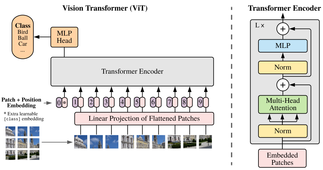
ViT模型原理如上图所示，其实ViT模型只是用了transformer的Encoder来提取特征（原始的transformer还有decoder部分，用于实现sequence to sequence，比如机器翻译）。下面将分别对各个部分做详细的介绍。

1.Patch Embedding

对于ViT来说，首先要将原始patch形式的2-D图像转换成一系列1-D的patch embeddings，这就好似NLP中的word embedding。输入的2-D图像记为$\mathbf{x} \in \mathbb{R}^{H \times W \times C}$,其中$H$和$W$分别是图像的高和宽，而$C$为通道数，对于RGB图像为3。如果将图像分为大小为$P \times P$的patchs,可以通过reshape等操作得到一系列patchs：$\mathbf{x}{p} \in \mathbb{R}^{N \times\left(P^{2} \cdot C\right)}$ ,总共可以得到的patch数是$N=H W / P^{2}$,这个就是序列的长度。注意这里直接将patch拉平为1-D，其特征大小为$P^{2} \cdot C$ .然后通过一个简单的线性变换将patchs映射成D大小的维度，这就是patch embeddings:$\mathbf{x}{\mathbf{p}}^{\prime} \in \mathbb{R}^{N \times D}$, 在实现上等同于对于x进行一个$P \times P$ 且stride为$P$ 的卷积操作。下面是具体的实现代码：

class PatchEmbed(nn.Module):
    """ Image to Patch Embedding
    """
    def __init__(self, img_size=224, patch_size=16, in_chans=3, embed_dim=768):
        super().__init__()
        img_size = to_2tuple(img_size)
        patch_size = to_2tuple(patch_size)
        num_patches = (img_size[1] // patch_size[1]) * (img_size[0] // patch_size[0])
        self.img_size = img_size
        self.patch_size = patch_size
        self.num_patches = num_patches

        self.proj = nn.Conv2d(in_chans, embed_dim, kernel_size=patch_size, stride=patch_size)

    def forward(self, x):
        B, C, H, W = x.shape
        # FIXME look at relaxing size constraints
        assert H == self.img_size[0] and W == self.img_size[1], \
            f"Input image size ({H}*{W}) doesn't match model ({self.img_size[0]}*{self.img_size[1]})."
        x = self.proj(x).flatten(2).transpose(1, 2)
        return x

2. Position Embedding

除了patch embeddings，模型还需要另外一个特殊的position embedding。transformer和CNN不同，需要position embedding来编码tokens的位置信息，这主要是因为self-attention是permutation-invariant，即打乱sequence里的tokens的顺序并不会改变结果。如果不给模型提供patch的位置信息，那么模型就需要通过patchs的语义来学习拼图，这就额外增加了学习成本。ViT论文中对比了几种不同的position embedding方案(如下），最后发现如果不提供positional embedding效果会差，但其它各种类型的positional embedding效果都接近，这主要是因为ViT的输入是相对较大的patchs而不是pixels，所以学习位置信息相对容易很多。

• 无positional embedding
• 1-D positional embedding：把2-D的patchs看成1-D序列
• 2-D positional embedding：考虑patchs的2-D位置（x, y）
• Relative positional embeddings：patchs的相对位置

在ViT中默认采用学习（训练的）的1-D positional embedding，在输入transformer的encoder之前直接将patch embeddings和positional embedding相加:

# 这里多1是为了后面要说的class token，embed_dim即patch embed_dim
self.pos_embed = nn.Parameter(torch.zeros(1, num_patches + 1, embed_dim)) 

# patch emded + pos_embed
x = x + self.pos_embed

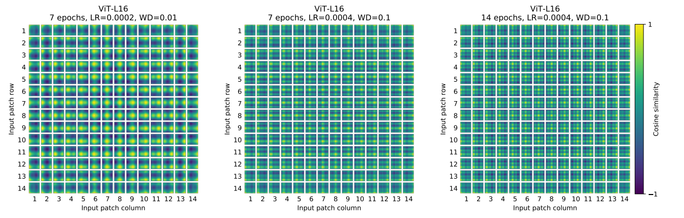
论文中也对学习到的positional embedding进行了可视化，发现相近的patchs的positional embedding比较相似，而且同行或同列的positional embedding也相近：

这里额外要注意的一点，如果改变图像的输入大小，ViT不会改变patchs的大小，那patch的数量$N$也会发生变化，那么之前学习的pos_embed就维度对不上了，ViT采用的方案是通过插值来解决这个问题。但是这种情形一般会造成性能少许损失，可以通过finetune模型来解决。另外最新的论文CPVT通过implicit Conditional Position encoding来解决这个问题（插入Conv来隐式编码位置信息，zero padding让Conv学习到绝对位置信息）。

3. Class Token

除了patch token，ViT借鉴BERT还增加了一个特殊的class token。后面会说，transformer的encoder输入是a sequence patch embeddings，输出也是同样长度的a sequence patch features，但图像分类最后需要获取image feature，简单的策略是采用pooling，比如求patch features的平均来获取image feature，但是ViT并没有采用类似的pooling策略，而是直接增加一个特殊的class token，其最后输出的特征加一个linear classifier就可以实现对图像的分类（ViT的pre-training时是接一个MLP head），所以输入ViT的sequence长度是$N+1$,class token对应的embedding在训练时随机初始化，然后通过训练得到，具体实现如下：

# 随机初始化
self.cls_token = nn.Parameter(torch.zeros(1, 1, embed_dim))

# Classifier head
self.head = nn.Linear(self.num_features, num_classes) if num_classes > 0 else nn.Identity()

# 具体forward过程
B = x.shape[0]
x = self.patch_embed(x)
cls_tokens = self.cls_token.expand(B, -1, -1)  # stole cls_tokens impl from Phil Wang, thanks
x = torch.cat((cls_tokens, x), dim=1)
x = x + self.pos_embed

4. Transformer Encoder

transformer最核心的操作就是self-attention，其实attention机制很早就在NLP和CV领域应用了，比如带有attention机制的seq2seq模型，但是transformer完全摒弃RNN或LSTM结构，直接采用attention机制反而取得了更好的效果：attention is all you need！简单来说，attention就是根据当前查询对输入信息赋予不同的权重来聚合信息，从操作上看就是一种“加权平均”。attention中共有3个概念：query, key和value，其中key和value是成对的，对于一个给定的query向量$q \in \mathbb{R}^{d}$,通过计算内积来匹配k个key向量(维度也是d,$K \in \mathbb{R}^{k \times d}$),得到的内积通过softmax来归一化得到k个权重，那么对于query其attention的输出就是k个key向量对应的value向量（即矩阵$V \in \mathbb{R}^{k \times d}$),对于一系列的N个query(即矩阵$Q \in \mathbb{R}^{N \times d}$)，可以通过矩阵计算它们的attention输出：

$$\operatorname{Attention}(Q, K, V)=\operatorname{Softmax}\left(\frac{Q K^{T}}{\sqrt{d_{k}}}\right) V$$

这里的$\sqrt{d_{k}}$为缩放因子以避免点击带来的方差影响。上述的Attention机制称为Scaled dot product attention，其实attention机制的变种有很多，但基本原理是相似的。如果$Q,K,V$都是从一个包含$N$个向量的sequence($X \in \mathbb{R}^{N \times D}$)变换得到：

$$Q=X W_{Q}, K=X W_{K}, V=X W_{V}$$

那么此时就变成了self-attention，这个时候就有N个(key,value)对,self-attention是transformer最核心部分，self-attention其实就是输入向量之间进行相互attention来学习到新特征。前面说过我们已经得到图像的patch sequence，那么送入self-attention就能到同样size的sequence输出，只不过特征改变了。更进一步，transformer采用的是multi-head self-attention (MSA），所谓的MSA就是采用定义h个attention heads，即采用h个self-attention应用在输入sequence上，在操作上可以将sequence拆分成h个size为$N \times d$，这里$D=h d$,不同的heads得到的输出concat在一起然后通过线性变换得到最终的输出,size也是$N \times D$:

$$\operatorname{MSA}(\mathbf{z})=\left[\mathrm{SA}_{1}(z) ; \mathrm{SA}_{2}(z) ; \cdots ; \mathrm{SA}_{k}(z)\right] \mathrm{U}_{m s a} \quad \mathrm{U}_{m s a} \in \mathbb{R}^{k \cdot D_{h} \times D}$$

MSA的计算量是和$N^{2}$成比例的，所以ViT的输入是patch embeddings，而不是pixel embeddings，这有计算量上的考虑。在实现上，MSA是可以并行计算各个head的，具体代码如下：

class Attention(nn.Module):
    def __init__(self, dim, num_heads=8, qkv_bias=False, qk_scale=None, attn_drop=0., proj_drop=0.):
        super().__init__()
        self.num_heads = num_heads
        head_dim = dim // num_heads
    
        self.scale = qk_scale or head_dim ** -0.5

        self.qkv = nn.Linear(dim, dim * 3, bias=qkv_bias)
        self.attn_drop = nn.Dropout(attn_drop)
        self.proj = nn.Linear(dim, dim)
        # 这里包含了dropout
        self.proj_drop = nn.Dropout(proj_drop)

    def forward(self, x):
        B, N, C = x.shape
        qkv = self.qkv(x).reshape(B, N, 3, self.num_heads, C // self.num_heads).permute(2, 0, 3, 1, 4)
        q, k, v = qkv[0], qkv[1], qkv[2]   # make torchscript happy (cannot use tensor as tuple)

        attn = (q @ k.transpose(-2, -1)) * self.scale
        attn = attn.softmax(dim=-1)
        attn = self.attn_drop(attn)

        x = (attn @ v).transpose(1, 2).reshape(B, N, C)
        x = self.proj(x)
        x = self.proj_drop(x)
        return x

在transformer中，MSA后跟一个FFN（Feed-forward network），这个FFN包含两个FC层，第一个FC层将特征从维度D变换成4D，后一个FC层将特征从维度4D变成D，中间的非线性激活函数采用GeLU，其实这就是一个MLP，具体实现如下：

class Mlp(nn.Module):
    def __init__(self, in_features, hidden_features=None, out_features=None, act_layer=nn.GELU, drop=0.):
        super().__init__()
        out_features = out_features or in_features
        hidden_features = hidden_features or in_features
        self.fc1 = nn.Linear(in_features, hidden_features)
        self.act = act_layer()
        self.fc2 = nn.Linear(hidden_features, out_features)
        self.drop = nn.Dropout(drop)

    def forward(self, x):
        x = self.fc1(x)
        x = self.act(x)
        x = self.drop(x)
        x = self.fc2(x)
        x = self.drop(x)
        return x

那么一个完成transformer encoder block就包含一个MSA后面接一个FFN，其实MSA和FFN均包含和ResNet一样的skip connection，另外MSA和FFN后面都包含layer norm层，具体实现如下：

class Block(nn.Module):

    def __init__(self, dim, num_heads, mlp_ratio=4., qkv_bias=False, qk_scale=None, drop=0., attn_drop=0.,
                 drop_path=0., act_layer=nn.GELU, norm_layer=nn.LayerNorm):
        super().__init__()
        self.norm1 = norm_layer(dim)
        self.attn = Attention(
            dim, num_heads=num_heads, qkv_bias=qkv_bias, qk_scale=qk_scale, attn_drop=attn_drop, proj_drop=drop)
        # NOTE: drop path for stochastic depth, we shall see if this is better than dropout here
        self.drop_path = DropPath(drop_path) if drop_path > 0. else nn.Identity()
        self.norm2 = norm_layer(dim)
        mlp_hidden_dim = int(dim * mlp_ratio)
        self.mlp = Mlp(in_features=dim, hidden_features=mlp_hidden_dim, act_layer=act_layer, drop=drop)

    def forward(self, x):
        x = x + self.drop_path(self.attn(self.norm1(x)))
        x = x + self.drop_path(self.mlp(self.norm2(x)))
        return x

5. ViT

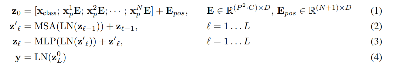
对于ViT模型来说，就类似CNN那样，不断堆积transformer encoder blocks，最后提取class token对应的特征用于图像分类，论文中也给出了模型的公式表达，其中（1）就是提取图像的patch embeddings，然后和class token对应的embedding拼接在一起并加上positional embedding；（2）是MSA，而（3）是MLP，（2）和（3）共同组成了一个transformer encoder block，共有L层；（4)是对class token对应的输出做layer norm，然后就可以用来图像分类。

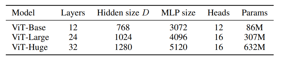
ViT模型的超参数主要包括以下，这些超参数直接影响模型参数以及计算量：

1. Layers：block的数量；
2. Hidden size D：隐含层特征，D在各个block是一直不变的；
3. MLP size：一般设置为4D大小；
4. Heads：MSA中的heads数量；
5. Patch size：模型输入的patch size，ViT中共有两个设置：14x14和16x16，这个只影响计算量；

类似BERT，ViT共定义了3中不同大小的模型：Base，Large和Huge，其对应的模型参数不同，如下所示。如ViT-L/16指的是采用Large结构，输入的patch size为16x16。类似BERT，ViT共定义了3中不同大小的模型：Base，Large和Huge，其对应的模型参数不同，如下所示。如ViT-L/16指的是采用Large结构，输入的patch size为16x16。

6. Experiments

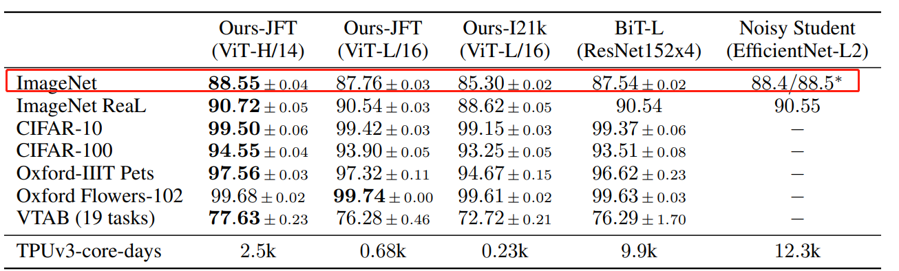
ViT并不像CNN那样具有inductive bias，论文中发现如果如果直接在ImageNet上训练，同level的ViT模型效果要差于ResNet，但是如果在比较大的数据集上petraining，然后再finetune，效果可以超越ResNet。比如ViT在Google私有的300M JFT数据集上pretrain后，在ImageNet上的最好Top-1 acc可达88.55%，这已经和ImageNet上的SOTA相当了（Noisy Student EfficientNet-L2效果为88.5%，Google最新的SOTA是Meta Pseudo Labels，效果可达90.2%）：

那么ViT至少需要多大的数据量才能和CNN旗鼓相当呢？这个论文也做了实验，结果如下图所示，从图上所示这个预训练所使用的数据量要达到100M时才能显示ViT的优势。transformer的一个特色是它的scalability：当模型和数据量提升时，性能持续提升。在大数据面前，ViT可能会发挥更大的优势。