Swin-transformer

论文信息： Swin Transformer: Hierarchical Vision Transformer using Shifted Windows
代码链接：https://github.com/microsoft/Swin-Transformer
整体信息： Swin Transformer 提出了一种针对视觉任务的通用的 Transformer 架构，Transformer 架构在 NLP 任务中已经算得上一种通用的架构，但是如果想迁移到视觉任务中有一个比较大的困难就是处理数据的尺寸不一样。作者分析表明，Transformer 从 NLP 迁移到 CV 上没有大放异彩主要有两点原因：(1)两个领域涉及的scale不同，NLP的scale是标准固定的，而CV的scale变化范围非常大。(2) CV比起NLP需要更大的分辨率，而且CV中使用Transformer的计算复杂度是图像尺度的平方，这会导致计算量过于庞大。为了解决这两个问题，Swin Transformer相比之前的ViT做了两个改进：1.引入CNN中常用的层次化构建方式构建层次化Transformer 2.引入locality思想，对无重合的window区域内进行self-attention计算。

swin

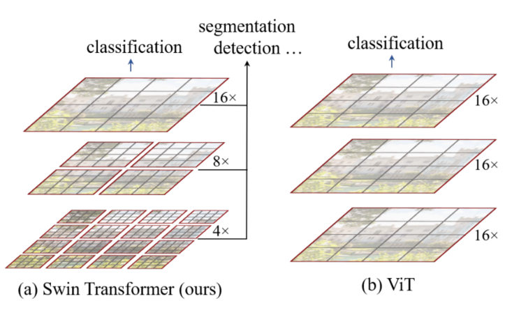
相比于ViT，Swin Transfomer计算复杂度大幅度降低，具有输入图像大小线性计算复杂度。Swin Transformer随着深度加深，逐渐合并图像块来构建层次化Transformer，可以作为通用的视觉骨干网络，应用于图像分类、目标检测、语义分割等任务。

1. 整体结构

我们先看下Swin Transformer的整体架构:

swin

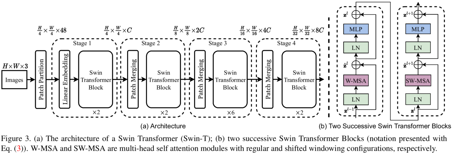
整个模型采取层次化的设计，一共包含4个Stage，每个stage都会缩小输入特征图的分辨率，像CNN一样逐层扩大感受野。

在输入开始的时候，做了一个Patch Embedding，将图片切成一个个图块，并嵌入到Embedding。
在每个Stage里，由Patch Merging和多个Block组成。
其中Patch Merging模块主要在每个Stage一开始降低图片分辨率。
而Block具体结构如右图所示，主要是LayerNorm，MLP，Window Attention 和 Shifted Window Attention组成 (为了方便讲解，我会省略掉一些参数)

class SwinTransformer(nn.Module):
    def __init__(...):
        super().__init__()
        ...
        # absolute position embedding
        if self.ape:
            self.absolute_pos_embed = nn.Parameter(torch.zeros(1, num_patches, embed_dim))
            
        self.pos_drop = nn.Dropout(p=drop_rate)

        # build layers
        self.layers = nn.ModuleList()
        for i_layer in range(self.num_layers):
            layer = BasicLayer(...)
            self.layers.append(layer)

        self.norm = norm_layer(self.num_features)
        self.avgpool = nn.AdaptiveAvgPool1d(1)
        self.head = nn.Linear(self.num_features, num_classes) if num_classes > 0 else nn.Identity()

    def forward_features(self, x):
        x = self.patch_embed(x)
        if self.ape:
            x = x + self.absolute_pos_embed
        x = self.pos_drop(x)

        for layer in self.layers:
            x = layer(x)

        x = self.norm(x)  # B L C
        x = self.avgpool(x.transpose(1, 2))  # B C 1
        x = torch.flatten(x, 1)
        return x

    def forward(self, x):
        x = self.forward_features(x)
        x = self.head(x)
        return x

其中有几个地方处理方法与ViT不同：

ViT在输入会给embedding进行位置编码。而Swin-T这里则是作为一个可选项（self.ape），Swin-T是在计算Attention的时候做了一个相对位置编码;

ViT会单独加上一个可学习参数，作为分类的token。而Swin-T则是直接做平均，输出分类，有点类似CNN最后的全局平均池化层;

2. Patch Embedding

在输入进Block前，我们需要将图片切成一个个patch，然后嵌入向量。具体做法是对原始图片裁成一个个 window_size * window_size的窗口大小，然后进行嵌入。这里可以通过二维卷积层，将stride，kernelsize设置为window_size大小。设定输出通道来确定嵌入向量的大小。最后将H,W维度展开，并移动到第一维度:

import torch
import torch.nn as nn


class PatchEmbed(nn.Module):
    def __init__(self, img_size=224, patch_size=4, in_chans=3, embed_dim=96, norm_layer=None):
        super().__init__()
        img_size = to_2tuple(img_size) # -> (img_size, img_size)
        patch_size = to_2tuple(patch_size) # -> (patch_size, patch_size)
        patches_resolution = [img_size[0] // patch_size[0], img_size[1] // patch_size[1]]
        self.img_size = img_size
        self.patch_size = patch_size
        self.patches_resolution = patches_resolution
        self.num_patches = patches_resolution[0] * patches_resolution[1]

        self.in_chans = in_chans
        self.embed_dim = embed_dim

        self.proj = nn.Conv2d(in_chans, embed_dim, kernel_size=patch_size, stride=patch_size)
        if norm_layer is not None:
            self.norm = norm_layer(embed_dim)
        else:
            self.norm = None

    def forward(self, x):
        # 假设采取默认参数
        x = self.proj(x) # 出来的是(N, 96, 224/4, 224/4) 
        x = torch.flatten(x, 2) # 把HW维展开，(N, 96, 56*56)
        x = torch.transpose(x, 1, 2)  # 把通道维放到最后 (N, 56*56, 96)
        if self.norm is not None:
            x = self.norm(x)
        return x

3.Patch Merging

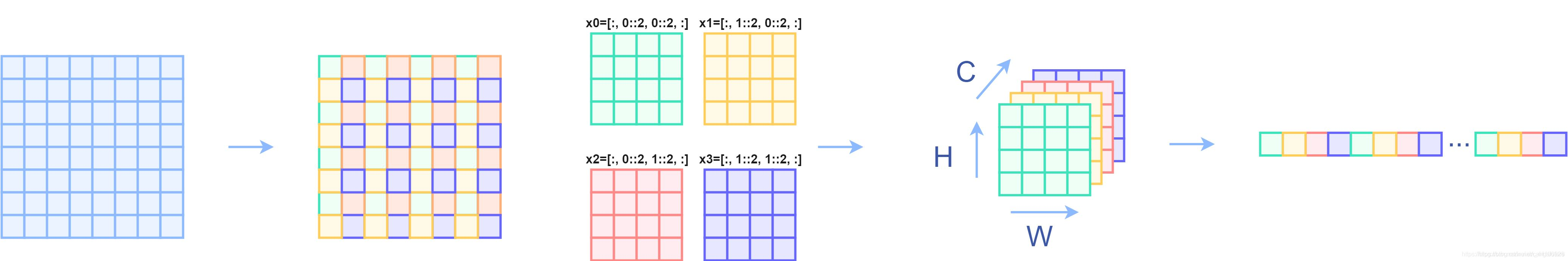
该模块的作用是在每个Stage开始前做降采样，用于缩小分辨率，调整通道数进而形成层次化的设计，同时也能节省一定运算量。在CNN中，则是在每个Stage开始前用stride=2的卷积/池化层来降低分辨率。每次降采样是两倍，因此在行方向和列方向上，间隔2选取元素。然后拼接在一起作为一整个张量，最后展开。此时通道维度会变成原先的4倍（因为H,W各缩小2倍），此时再通过一个全连接层再调整通道维度为原来的两倍.

class PatchMerging(nn.Module):
    def __init__(self, input_resolution, dim, norm_layer=nn.LayerNorm):
        super().__init__()
        self.input_resolution = input_resolution
        self.dim = dim
        self.reduction = nn.Linear(4 * dim, 2 * dim, bias=False)
        self.norm = norm_layer(4 * dim)

    def forward(self, x):
        """
        x: B, H*W, C
        """
        H, W = self.input_resolution
        B, L, C = x.shape
        assert L == H * W, "input feature has wrong size"
        assert H % 2 == 0 and W % 2 == 0, f"x size ({H}*{W}) are not even."

        x = x.view(B, H, W, C)

        x0 = x[:, 0::2, 0::2, :]  # B H/2 W/2 C
        x1 = x[:, 1::2, 0::2, :]  # B H/2 W/2 C
        x2 = x[:, 0::2, 1::2, :]  # B H/2 W/2 C
        x3 = x[:, 1::2, 1::2, :]  # B H/2 W/2 C
        x = torch.cat([x0, x1, x2, x3], -1)  # B H/2 W/2 4*C
        x = x.view(B, -1, 4 * C)  # B H/2*W/2 4*C

        x = self.norm(x)
        x = self.reduction(x)

        return x

下面是一个示意图（输入张量N=1, H=W=8, C=1，不包含最后的全连接层调整）

swin

3. Window Attention

这是这篇文章的关键。传统的Transformer都是基于全局来计算注意力的，因此计算复杂度十分高。而Swin Transformer则将注意力的计算限制在每个窗口内，进而减少了计算量。我们先简单看下公式：

$\operatorname{Attention}(Q, K, V)=\operatorname{SoftMax}\left(Q K^{T} / \sqrt{d}+B\right) V$

主要区别是在原始计算Attention的公式中的Q,K时加入了相对位置编码。后续实验有证明相对位置编码的加入提升了模型性能。

4. Shifted Window Attention

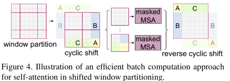
前面的Window Attention是在每个窗口下计算注意力的，为了更好的和其他window进行信息交互，Swin Transformer还引入了shifted window操作。

swin

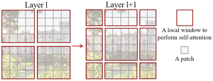
左边是没有重叠的Window Attention，而右边则是将窗口进行移位的Shift Window Attention。可以看到移位后的窗口包含了原本相邻窗口的元素。但这也引入了一个新问题，即window的个数翻倍了，由原本四个窗口变成了9个窗口。在实际代码里，我们是通过对特征图移位，并给Attention设置mask来间接实现的。能在保持原有的window个数下，最后的计算结果等价。

swin

4.1 特征图移位操作

代码里对特征图移位是通过torch.roll来实现的，下面是示意图

swin

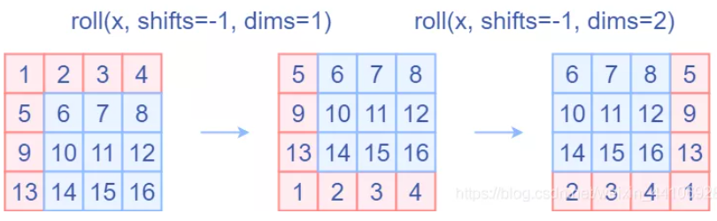
第一位操作是针对行进行移位，第二位操作时针对列进行移位操作。如果需要reverse cyclic shift的话只需把参数shifts设置为对应的正数值。

4.2 attention mask

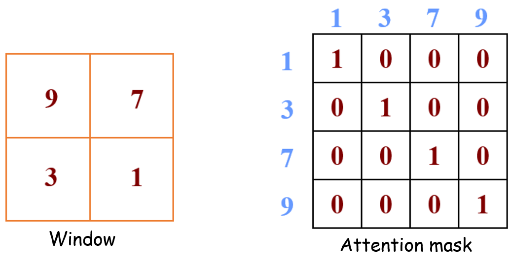
我认为这是Swin Transformer的精华，通过设置合理的mask，让Shifted Window Attention在与Window Attention相同的窗口个数下，达到等价的计算结果。首先我们对Shift Window后的每个窗口都给上index，并且做一个roll操作（window_size=2, shift_size=1）

swin

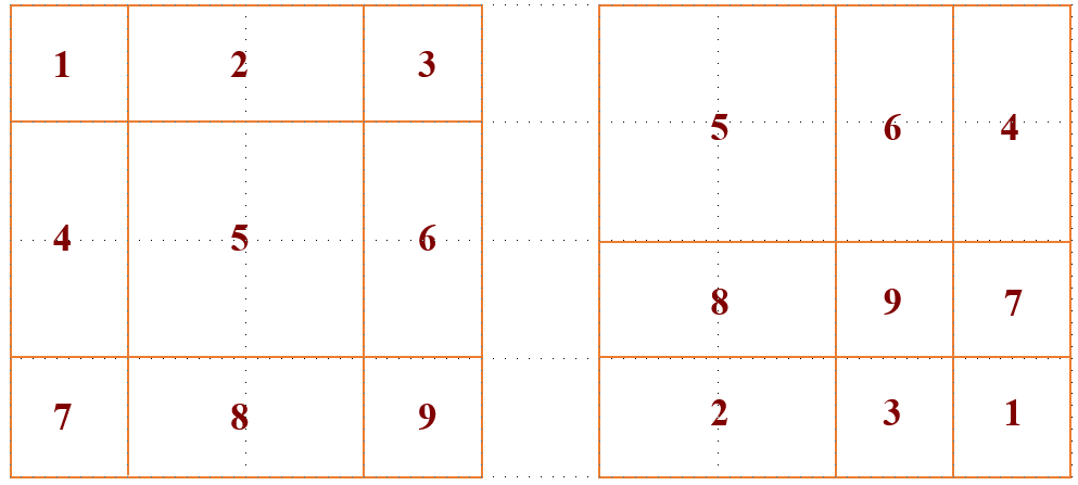
我们希望在计算Attention的时候，让具有相同index QK进行计算，而忽略不同index QK计算结果。最后正确的结果如下图所示.

例1：比如右上角这个 window，如下图所示。它由4个 patch 组成，所以应该计算出的 attention map是4×4的。但是6和4是2个不同的 sub-window，我们又不想让它们的 attention 发生交叠。所以我们希望的 attention map 和attention mask如下图所示。

swin

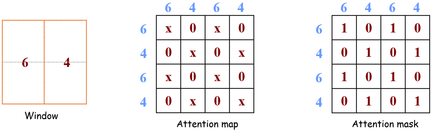
例2：比如右下角这个 window，对应的 attention map 和attention mask是下面这个样子。

swin

5. transformer block 整体结构

swin

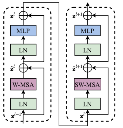
两个连续的Block架构如上图所示，需要注意的是一个Stage包含的Block个数必须是偶数，因为需要交替包含一个含有Window Attention的Layer和含有Shifted Window Attention的Layer。我们看下Block的前向代码：

def forward(self, x):
    H, W = self.input_resolution
    B, L, C = x.shape
    assert L == H * W, "input feature has wrong size"

    shortcut = x
    x = self.norm1(x)
    x = x.view(B, H, W, C)

    # cyclic shift
    if self.shift_size > 0:
        shifted_x = torch.roll(x, shifts=(-self.shift_size, -self.shift_size), dims=(1, 2))
    else:
        shifted_x = x

    # partition windows
    x_windows = window_partition(shifted_x, self.window_size)  # nW*B, window_size, window_size, C
    x_windows = x_windows.view(-1, self.window_size * self.window_size, C)  # nW*B, window_size*window_size, C

    # W-MSA/SW-MSA
    attn_windows = self.attn(x_windows, mask=self.attn_mask)  # nW*B, window_size*window_size, C

    # merge windows
    attn_windows = attn_windows.view(-1, self.window_size, self.window_size, C)
    shifted_x = window_reverse(attn_windows, self.window_size, H, W)  # B H' W' C

    # reverse cyclic shift
    if self.shift_size > 0:
        x = torch.roll(shifted_x, shifts=(self.shift_size, self.shift_size), dims=(1, 2))
    else:
        x = shifted_x
    x = x.view(B, H * W, C)

    # FFN
    x = shortcut + self.drop_path(x)
    x = x + self.drop_path(self.mlp(self.norm2(x)))

    return x

整体流程如下：

先对特征图进行LayerNorm
通过self.shift_size决定是否需要对特征图进行shift
然后将特征图切成一个个窗口
计算Attention，通过self.attn_mask来区分Window Attention还是Shift Window Attention
将各个窗口合并回来
如果之前有做shift操作，此时进行reverse shift，把之前的shift操作恢复
做dropout和残差连接
再通过一层LayerNorm+全连接层，以及dropout和残差连接

6. experiments

swin

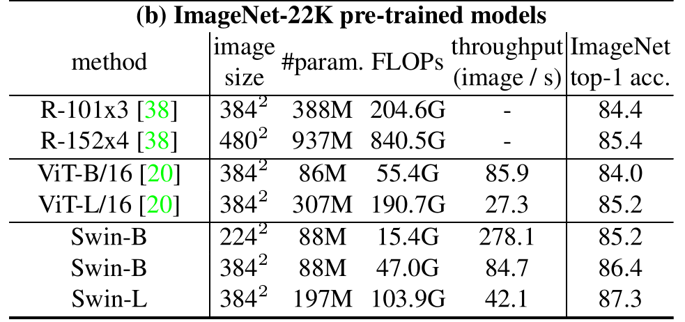
在ImageNet22K数据集上，准确率能达到惊人的86.4%。另外在检测，分割等任务上表现也很优异，感兴趣的可以翻看论文最后的实验部分。

7. conclusion

这篇文章创新点很棒，引入window这一个概念，将CNN的局部性引入，还能控制模型整体计算量。在Shift Window Attention部分，用一个mask和移位操作，很巧妙的实现计算等价。