MeanShift最初由Fukunaga和Hostetler在1975年提出,但是一直到2000左右这篇PAMI的论文Mean Shift: A Robust Approach Toward Feature Space Analysis,将它的原理和收敛性等重新整理阐述,并应用于计算机视觉和图像处理领域之后,才逐渐为人熟知。在了解mean-shift算法之前,先了解一下概率密度估计的概念。
概率密度估计
密度估计是指有给定样本集和求解随机变量的分布密度函数,解决这一问题的方法包括:参数估计和非参数估计。
参数估计:在我们已经知道观测数据符合某些模型的情况下,我们可以利用参数估计的方法来确定这些参数值,然后得出概率密度模型。前提是观测数据服从一个已知概率密度函数。
非参数估计:无需任何先验知识完全依靠特征空间中样本点计算其密度估计值.可以处理任意概率分布,不必假设服从已知分布;常用的无参数密度估计方法有:直方图法、最近邻域法和核密度估计法。MeanShift算法正属于核密度估计法。无需任何先验知识完全依靠特征空间中样本点计算其密度估计值。
核密度估计
mean shift算法使用核函数估计样本密度,假设对于大小为$n$,维度为$d$ 的数据集,$D=\left{x{1}, x{2}, x{3}, \ldots x{n}\right}, D \in R^{d}$ ,核函数K的带宽为h,则该函数的核密度估计为:
定义满足核函数条件为:
其中,$c_{k,d}$ 系数是归一化常数,使得$K(x)$ 的积分为1.
常见的核函数有高斯核函数,其形式如下:
其中,h称为带宽(bandwidth),不同带宽的核函数如下图所示:
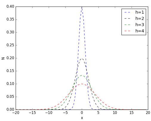
从高斯函数的图像可以看出,当带宽h一定时,样本点之间的距离越近,其核函数的值越大,当样本点之间的距离相等时,随着高斯函数的带宽h的增加,核函数的值在减小。高斯核的python实现如下:
1 | import numpy as np |
以高斯核估计一维数据集的密度为例,每个样本点都设置以该样本为中心的高斯分布,累加所有高斯分布,就得到该数据集的密度。
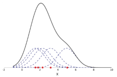
其中虚线表示每个样本点的高斯核,实现表示累加后所有样本高斯核后的数据集密度。
mean-shift 算法理论
朴素mean-shift向量形式
对于给定的d维度空间中的n个样本点$\left{x{1}, x{2}, x{3}, \ldots x{n}\right}$ ,则对于x点,其mean-shift向量的基本形式为:
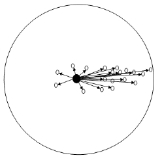
其中$S_h$指的是一个半径为h的高维球区域,如上图中的圆形区域。$S_h$的定义为:
里面所有点与圆心为起点形成的向量相加的结果就是Mean shift向量。下图黄色箭头就是 $M_h$ (mean-shift 向量)。
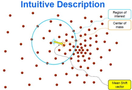
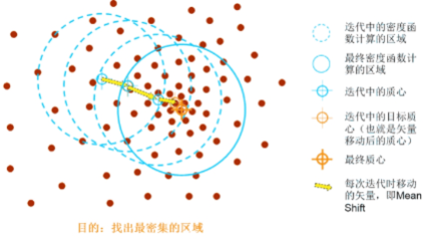
对于Mean Shift算法,是一个迭代的步骤,即先算出当前点的偏移均值,将该点移动到此偏移均值,然后以此为新的起始点,继续移动,直到满足最终的条件。
引入核函数的Mean Shift向量形式
Mean Shift算法的基本目标是将样本点向局部密度增加的方向移动,我们常常所说的均值漂移向量就是指局部密度增加最快的方向。上节通过引入高斯核可以知道数据集的密度,梯度是函数增加最快的方向,因此,数据集密度的梯度方向就是密度增加最快的方向。
高斯核:$K(x)=c_{k, d} k\left(|x|^{2}\right)$
其中$g(s)=-k^{\prime}(s)$ ,上式的第一项为实数值。
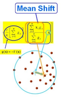
因此第二项的向量方向与梯度方向一致,第二项的表达式为:
上式的含义就是本篇文章的主题:均值漂移。由上式推导可知:均值漂移向量所指的方向是密度增加最大的方向。
要使$\nabla f(x)=0$ ,当且仅当$m_{h}(\mathrm{x})=0$ ,可以得出新坐标:
因此,Mean Shift算法流程为:
(1)计算每个样本的均值漂移向量 $m_{h}(\mathrm{x})$ ;
(2)对每个样本点以 $m{h}(\mathrm{x})$ 进行平移,即:$x=x+m{h}(x)$ ;
(3)重复(1)(2),直到样本点收敛,即:$m_{h}(\mathrm{x})<\varepsilon$ (人工设定)或者迭代次数小于设定值;
(4)收敛到相同点的样本被认为是同一簇类的成员;
mean-shift应用
聚类
Mean-Shift聚类就是对于集合中的每一个元素,对它执行下面的操作:把该元素移动到它邻域中所有元素的特征值的均值的位置,不断重复直到收敛。准确的说,不是真正移动元素,而是把该元素与它的收敛位置的元素标记为同一类。在实际中,为了加速,初始化的时候往往会初始化多个窗口,然后再进行聚类。
对应python的实现如下:
1 | import numpy as np |
以上代码实现了基本的流程,但是执行效率很慢,正式使用时建议使用scikit-learn库中的MeanShift。scikit-learn 中mean-shift的使用方法:
1 | import numpy as np |
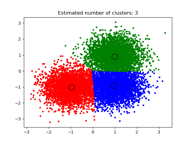
运行结果如下:
number of estimated clusters : 3
图像分割
对于图像分割,最简单直接的方法就是对图像上每个点的像素值进行聚类。我们对下图的像素点映射为RGB三维空间:
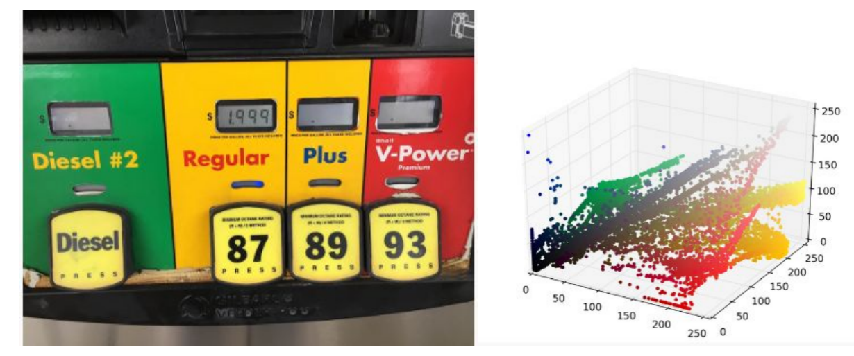
每个样本点最终会移动到核概率密度的峰值,移动到相同峰值的样本点属于同一种颜色,下图给出图像分割结果:

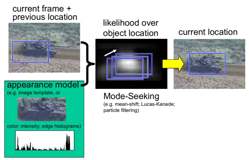
目标跟踪
基于meanshift的目标跟踪算法通过分别计算目标区域和候选区域内像素的特征值概率得到关于目标模型和候选模型的描述,然后利用相似函数度量初始帧目标模型和当前帧的候选模版的相似性,选择使相似函数最大的候选模型并得到关于目标模型的Meanshift向量,这个向量正是目标由初始位置向正确位置移动的向量。由于均值漂移算法的快速收敛性,通过不断迭代计算Meanshift向量,算法最终将收敛到目标的真实位置,达到跟踪的目的。